
Real estate investment success depends on more than just good instincts—it requires precise understanding of performance metrics that reveal true asset value and management capability. In today’s market, where the U.S. price-to-income ratio has reached 4.97, both sponsors and investors need clear frameworks to evaluate opportunities.
For Investors: These metrics form the foundation for evaluating potential investment partners and opportunities. Understanding each measurement helps you assess not just returns, but how managers approach valuation, risk management, and investor protection.
For Sponsors: These calculations demonstrate your ability to create and protect value. Strong command of these metrics signals institutional-quality operations and builds investor confidence through every stage of the investment lifecycle.
The following analysis examines 10 of the most critical real estate return measurements, providing both sponsors and investors with the tools needed to make informed decisions in today’s complex market environment.
Net Operating Income (NOI)
Net Operating Income measures property performance through revenue and expense analysis. Property owners and lenders rely on NOI calculations to assess operational profitability.
NOI Definition and Formula
NOI calculations show income after operating expenses but before financing costs and taxes. The standard formula reads:
NOI = Total Operating Income – Operating Expenses
Rental revenue forms the primary income component, supplemented by parking fees and service charges. The metric excludes debt payments, capital expenses, depreciation, and amortization costs.
NOI Calculation Steps
Property analysis requires two main components:
- Income Assessment
- Potential rental income
- Vacancy allowances
- Additional revenue streams (parking, amenities)
- Operating Expenses Evaluation
- Property tax obligations
- Insurance costs
- Maintenance requirements
- Utility expenses
- Management fees
NOI Limitations and Uses
Lenders examine NOI to determine debt service capability. The metric helps calculate capitalization rate, showing profitability against total investment.
NOI calculations exclude several crucial elements:
- Mortgage payments
- Capital improvements
- Tax obligations
- Market changes
The measurement assumes cash purchases, though most acquisitions involve financing. NOI accuracy depends on precise income and expense reporting. The metric proves most valuable alongside other performance indicators, offering clear insights into operational performance.
- For Investors: NOI provides your clearest view into a property’s fundamental earning power, stripped of financing decisions and tax implications.
- For Sponsors: Strong NOI tracking demonstrates your operational efficiency and helps justify valuation assumptions to potential investors.
Cash Flow
Cash flow analysis reveals property performance through actual money movement patterns. The metric shows real-time financial health, offering concrete data for investment decisions.
Cash Flow Components
Two distinct streams shape property cash flow: income and expenses. Monthly rental payments create the primary income base, while pet fees, parking charges, and application fees generate supplemental revenue. A 50-unit property charging USD 1,000 per unit produces USD 50,000 monthly gross income.
Operating expenses include:
- Management fees (8-10% of rental income)
- Repairs and maintenance costs
- Insurance coverage
- Property tax obligations
- Utility payments
Cash Flow Analysis Methods
Cash flow calculations follow clear steps. The process starts with gross income, subtracts operating expenses for NOI, then removes debt service to determine Cash Flow Before Tax.
Monthly NOI of USD 30,000 yields USD 28,500 in distributable income after a 5% reserve allocation (USD 1,500). Debt service coverage ratio helps predict sustained positive cash flow against mortgage obligations.
Cash Flow Optimization Strategies
Property owners employ tested methods to maximize cash flow. Annual lease structures with 3% rent escalations create predictable income growth.
Strategic expense management protects cash flow. HVAC and plumbing maintenance prevents emergency repair costs. Property tax appeals during market corrections produce substantial savings.
Revenue expansion opportunities exist throughout properties. Storage unit conversions and vending machine installations generate new income sources. These additions boost tenant satisfaction while reducing turnover expenses.
- For Investors: Cash flow analysis reveals how effectively managers convert property income into actual returns for investors.
- For Sponsors: Detailed cash flow management showcases your ability to maintain property performance while meeting investor distribution expectations.
Capitalization Rate
Capitalization rate calculations determine property values through income analysis . The metric converts net operating income into value estimates, providing crucial return indicators.
Cap Rate Fundamentals
Cap rate calculations divide net operating income by current market value. A USD 14 million property generating USD 600,000 NOI shows a 4.3% cap rate. This percentage reveals expected unlevered returns.
The metric functions similarly to stock market price-to-earnings ratios. Investors match property cap rates against return requirements, weighing income potential against market risks.
Cap Rate Market Benchmarks
January 2023 data from the National Association of Realtors shows distinct market patterns:
| Property Type | Cap Rate |
| Multifamily | 4.9% |
| Office | 6.9% |
| Industrial | 6.2% |
| Retail | 6.7% |
Commercial property cap rates stay within 500 basis points since 2001, averaging 6.29% with 1.12% standard deviation. Property type correlations exceed .95.
Cap Rate Risk Assessment
Higher cap rates signal elevated risk and return potential, while lower rates suggest stability with modest yields. Market factors shape these patterns:
Location quality drives cap rate variations. Prime areas command lower rates through stable demand and employment strength. Transit access and employment centers influence risk assessments.
Economic conditions guide cap rate movements. Strong GDP growth and low unemployment correlate with compressed cap rates. Interest rate changes affect cap rate expansion and compression.
Cap rates show consistency across sectors, though hotel properties broke patterns in early 2010s amid short-term rental growth. Market structure changes create notable metric variations.
- For Investors: Cap rates help you compare opportunities across markets and property types while indicating relative risk levels.
- For Sponsors: Clear cap rate analysis demonstrates your market expertise and ability to identify value opportunities.
Cash-on-Cash Return
Cash-on-cash return calculations cut through financing complexities to show actual cash efficiency . The metric reveals yearly cash yield against initial investment dollars, offering clarity for leveraged acquisitions.
Cash-on-Cash Return Formula
The formula weighs annual pre-tax cash flow against total cash invested. Property financing structures shape this measurement, making it vital for leveraged investments. Key components include:
Annual Pre-Tax Cash Flow = Net Operating Income – Annual Debt Service Total Cash Invested = Down Payment + Closing Costs + Initial Repairs
A USD 500,000 acquisition using USD 250,000 cash produces USD 15,000 pre-tax cash flow (USD 25,000 NOI minus USD 10,000 mortgage interest), showing 6% cash-on-cash return.
Cash-on-Cash Return Analysis
Market participants seek 8% to 12% cash-on-cash returns, adjusting expectations with market cycles and asset classes. Leveraged property evaluation benefits particularly from this metric, versus all-cash purchases.
Performance comparison shows:
| Financing Structure | Property Value | Equity | NOI | Debt Service | Cash-on-Cash Return |
| Leveraged | USD 6M | USD 2M | USD 400K | USD 200K | 10% |
| All-Cash | USD 6M | USD 6M | USD 400K | USD 0 | 6.7% |
Cash-on-Cash Return Limitations
The metric shows specific boundaries in analysis. First-year cash flows dominate calculations, missing future income and expense shifts. Notable exclusions include:
- Tax impact on actual yields
- Property value growth
- Future capital needs
- Exit proceeds
Return calculations might show inflated yields when capital returns mix with income returns. Prime markets often accept lower cash-on-cash returns, trading immediate yield for stronger market fundamentals.
- For Investors: This metric shows exactly how much cash you’ll receive relative to your investment, helping evaluate actual returns against alternatives.
- For Sponsors: Strong cash-on-cash performance proves your ability to generate meaningful investor distributions from day one.
Debt Service Coverage Ratio
Image Source: Career Principles
DSCR calculations determine loan viability through income-to-debt analysis . Lenders use this metric to assess property debt capacity and financial stability.
DSCR Calculation Method
DSCR measures income against debt obligations. A property showing USD 450,000 NOI with USD 250,000 debt service produces 1.8 DSCR, yielding USD 1.80 income per USD 1.00 debt service.
Key calculation elements include:
- Net Operating Income
- Debt Service Requirements
- Property Tax Obligations
- Insurance Costs
- Association Dues
DSCR Industry Standards
Commercial lenders mandate minimum DSCR between 1.20 and 1.25. Properties must generate 25% excess income above debt obligations. Standards show property-specific variations:
| Property Category | Typical Minimum DSCR |
| Multifamily | 1.20 |
| Commercial | 1.25 |
| Retail | 1.25-1.30 |
| Industrial | 1.25-1.50 |
DSCR Risk Indicators
Strong DSCR numbers signal robust financial performance. Ratios below 1.0 indicate insufficient income for debt coverage. These situations demand personal capital injections for debt service.
Risk evaluation considers:
- Occupancy stability
- Rental rate movements
- Operating cost changes
- Interest rate shifts
DSCR trends reveal potential financial stress. Lenders examine individual properties and portfolio-wide metrics during underwriting. Global DSCR analysis shows interest rate sensitivity, particularly crucial for adjustable-rate debt structures.
- For Investors: DSCR indicates how well protected your investment is from potential market downturns or income fluctuations.
- For Sponsors: Solid DSCR numbers demonstrate your conservative approach to leverage and focus on investor capital protection.
Internal Rate of Return
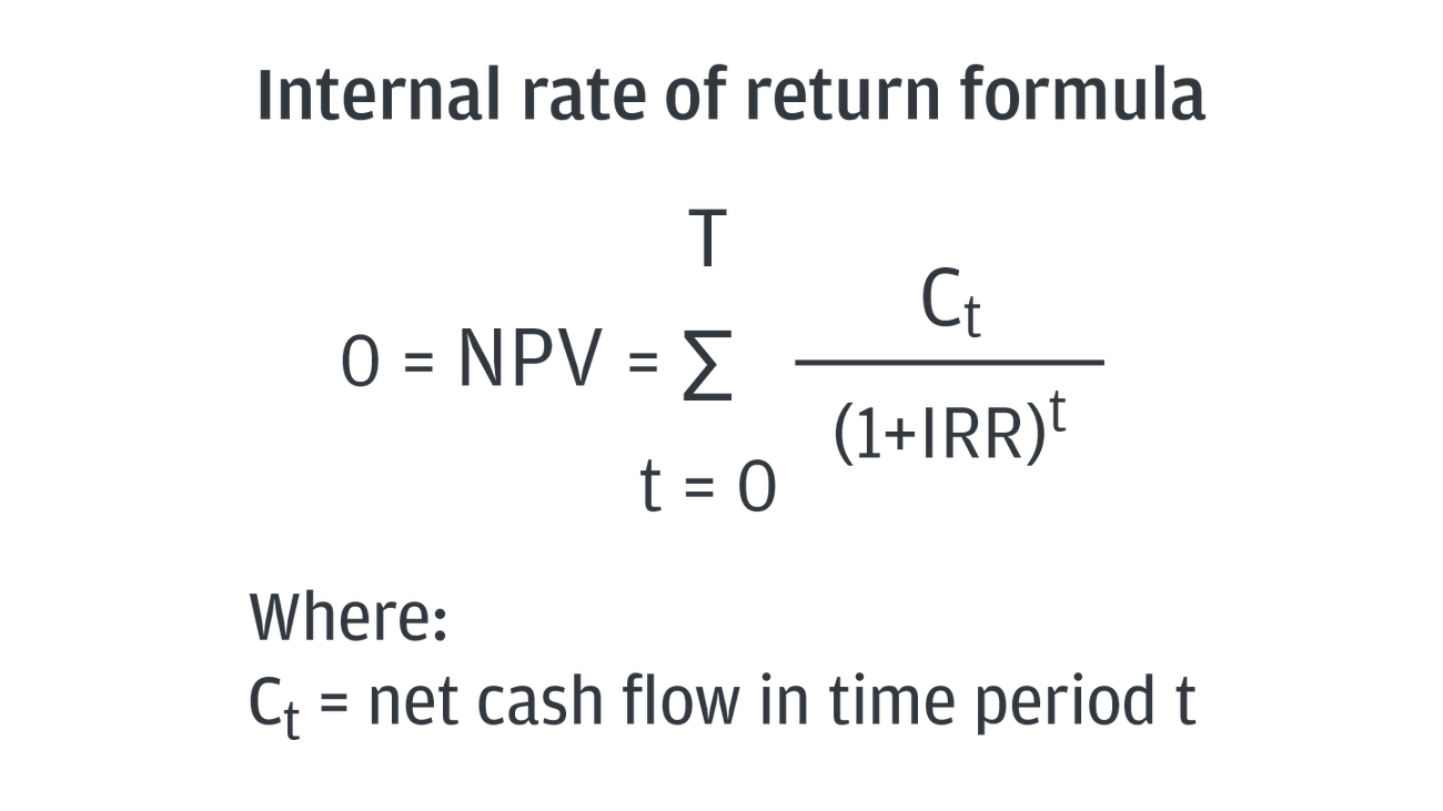
Image Source: J.P. Morgan
IRR calculations reveal time-adjusted investment performance . The metric shows annualized compound returns, surpassing basic cash flow measurements.
IRR Calculation Approach
IRR finds the discount rate zeroing net present value of all cash flows. Essential components include:
- Initial capital outlay
- Period-by-period cash flows
- Exit value projections
Excel functions simplify complex IRR mathematics. The calculations weigh both cash flow timing and size, showing complete investment results.
IRR Investment Applications
IRR guides strategic property decisions. The metric excels with irregular cash flow patterns. Global real estate fund data shows peak IRR performance during 2011-2016, with 2013 vintages reaching 18.39%.
Key metric distinctions:
- Time value focus versus ROI
- Multiple cash flow periods versus CAGR
- Full lifecycle view versus cap rate
IRR Performance Benchmarks
Quality investments typically achieve 18-20% IRR. Strategy types show distinct ranges:
| Investment Type | Target IRR Range |
| Core | 8-10% |
| Value-Add | 11-15% |
| Opportunistic | 16%+ |
IRR shows specific limitations. The metric assumes constant reinvestment rates. Hold period variations and initial investment differences might skew results. Proper analysis pairs IRR with complementary performance measures.
- For Investors: IRR helps you understand the true time-value impact of your investment, especially important for longer-term holds.
- For Sponsors: Strong IRR tracking demonstrates your ability to manage both ongoing distributions and successful exit timing.
Equity Multiple
Equity multiple calculations quantify lifetime investment returns . The metric shows total return multiples against initial capital deployment.
Equity Multiple Basics
Total cash distributions divided by total equity invested yields the equity multiple. The calculation answers direct value creation questions. USD 2 million equity generating USD 4.6 million total distributions produces 2.3x equity multiple.
Core measurement elements include:
- Total Cash Distributions: Operating profits plus sale proceeds
- Total Capital Invested: Initial equity and subsequent contributions
Equity Multiple Analysis
Raw return measurements distinguish equity multiple from time-weighted metrics. Double investment value shows 2.0x multiple, independent of time period.
Property sector results demonstrate typical outcomes:
| Investment Type | Initial Equity | Total Return | Equity Multiple |
| Multifamily | USD 250,000 | USD 475,000 | 1.9x |
| Commercial | USD 1,000,000 | USD 2,500,000 | 2.5x |
Equity Multiple Targets
Core properties target 1.5x to 2.0x multiples across 5-7 year holds. Value-add strategies push 2.0x to 3.0x multiples through shorter periods.
Target selection factors include:
- Current market dynamics
- Risk-return relationships
- Investment duration
IRR calculations pair naturally with equity multiple analysis. IRR shows yearly performance while equity multiple reveals total value growth. Three-month investments showing 30% IRR might yield 1.075x multiples, while five-year holds at 15% IRR reach 2.0x multiples.
- For Investors: This straightforward metric shows exactly how much your investment grows over the entire hold period.
- For Sponsors: Clear equity multiple targets demonstrate your focus on total investor returns, not just annual distributions.
Preferred Return
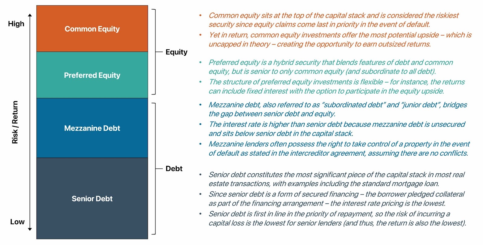
Image Source: Wall Street Prep
Preferred return structures establish profit distribution hierarchies in real estate partnerships . The metric sets precise payment priorities among capital partners, creating clear distribution waterfalls.
Preferred Return Structure
Two distinct structures govern preferred returns. True preferred returns grant priority payments to specific investors, while pari-passu arrangements allow concurrent distributions. Preferred equity maintains capital stack seniority, securing first position in distribution schedules.
Standard structures show:
| Return Type | Distribution Priority | Common Range |
| True Preferred | Investors First | 6-8% |
| Pari-passu | Simultaneous | 8-10% |
| Participating | Shared Excess | Variable |
Preferred Return Calculations
Return calculations follow established protocols. Agreements often specify cumulative provisions beyond base returns. An 8% preferred return on USD 1 million requires USD 80,000 annual threshold payments.
Two distinct methods apply:
- Simple Interest: Unpaid returns create direct obligations
- Compound Interest: Missed payments add to capital base
Preferred Return Impact
Preferred returns shape investment structures. Limited partners gain distribution priority protection. Properties yielding 7% against 8% preferred hurdles carry 1% deficits into subsequent periods.
Sponsor-investor alignment strengthens through preferred structures. Performance incentives motivate sponsors to exceed preferred thresholds. Waterfall structures showing 75/25 splits above 8% preferred returns grant investors 75% of excess profits.
Distribution mechanics influence:
- Risk allocation methods
- Payment schedules
- Sponsor incentives
- Investment viability
- For Investors: Preferred returns provide clarity on distribution priority and downside protection for your capital.
- For Sponsors: Well-structured preferred returns show your commitment to investor alignment and transparent profit sharing.
Total Return
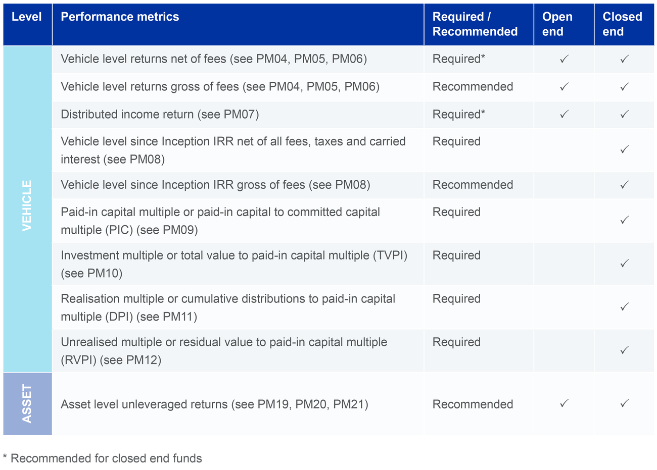
Image Source: INREV
Total return metrics reveal complete investment performance through income and appreciation analysis . Market participants track both current yields and value changes for accurate performance measurement.
Total Return Components
Total return combines income generation and capital appreciation. Revenue streams include:
- Fixed-income investment yields
- Operating cash distributions
- REIT dividend payments
Market value changes drive capital appreciation. Performance example: 5% annual yield across three years plus 20% disposition gain creates 35% total return.
Total Return Analysis
Performance tracking demands fixed and variable component measurement. Return elements show distinct patterns:
| Return Element | Characteristics | Impact |
| Income Payments | Fixed, Definitive | Immediate Returns |
| Capital Gains | Variable, Potential | Future Growth |
Dividend reinvestment shapes long-term results. Standard calculation methods use:
Total Return = ((Ending Value + Distributions) / Beginning Value) – 1
Total Return Optimization
Return enhancement requires strategic focus. Key areas include:
- Income Management
- Rental rate strategy
- Cost controls
- Distribution policies
- Value Creation
- Asset improvements
- Cycle positioning
- Location advantages
Performance monitoring requires both yearly and cumulative analysis. Twelve-month measurements show annual results while investment-period tracking reveals total gains.
- For Investors: Total return combines all value creation elements, helping you evaluate manager performance comprehensively.
- For Sponsors: Strong total returns demonstrate your ability to create value through both operations and market positioning.
Cumulative Return
Cumulative return measurements show total investment value changes across hold periods . The metric reveals aggregate performance rather than yearly results.
Cumulative Return Measurement
Basic calculations subtract initial value from final value, divided by initial investment. USD 100,000 growing to USD 200,000 demonstrates 100% cumulative return.
Key measurement elements include:
- Starting capital
- Final asset value
- Reinvested earnings
- Capital appreciation
Property calculations combine operating income and value growth. Percentage expressions distinguish cumulative returns from equity multiples.
Cumulative Return Analysis
Performance evaluation focuses on total results independent of time. Long-term assessment benefits from this approach. USD 10,000 reaching USD 11,229 shows 112.29% cumulative return.
Analysis requires tracking:
- Value fluctuations
- Income streams
- Operating costs
- Capital needs
Long-term holdings demonstrate metric strengths. Extended periods often show higher cumulative returns versus annualized figures.
Cumulative Return Applications
Investment analysis uses cumulative returns for:
| Application | Purpose | Benefit |
| Portfolio Evaluation | Track total gains | Clear performance picture |
| Investment Comparison | Assess relative success | Direct value comparison |
| Risk Assessment | Measure total exposure | Long-term perspective |
Total growth measurement proves valuable. Duration context enhances return comparisons.
Applications extend to:
- Strategy evaluation
- Asset comparison
- Portfolio planning
- Risk analysis
Wealth creation tracking benefits from this metric. Time-based metrics provide essential context for return analysis.
- For Investors: This metric helps you understand total portfolio impact across your entire investment period.
- For Sponsors: Cumulative returns showcase your long-term value creation capability across market cycles.
Comparison Table
| Metric | Definition/Purpose | Primary Formula/Calculation | Typical Target Range | Key Limitations/Considerations |
| Net Operating Income (NOI) | Measures property’s operational profitability before financing costs and taxes | Total Operating Income – Operating Expenses | Varies by property type | Excludes debt service, capital expenditures, and income taxes |
| Cash Flow | Measures actual money movement through property operations | NOI – Debt Service | Positive monthly cash flow | Excludes tax implications and future capital needs |
| Capitalization Rate | Converts NOI into property value estimate | NOI ÷ Current Market Value | 4.9% – 6.9% (varies by property type) | Assumes stabilized operations and all-cash purchase |
| Cash-on-Cash Return | Measures annual return relative to cash invested | Annual Pre-Tax Cash Flow ÷ Total Cash Invested | 8% – 12% | Only considers first-year cash flows; excludes appreciation |
| Debt Service Coverage Ratio | Evaluates property’s ability to cover debt payments | NOI ÷ Total Debt Service | 1.20 – 1.50 (varies by property type) | Sensitive to interest rate changes and income fluctuations |
| Internal Rate of Return | Measures annualized effective compounded return | Net Present Value of All Cash Flows = 0 | 8% – 20% (varies by strategy) | Assumes reinvestment at same rate; complex calculation |
| Equity Multiple | Shows total return relative to initial investment | Total Cash Distributions ÷ Total Equity Invested | 1.5x – 3.0x | Doesn’t account for time value of money |
| Preferred Return | Establishes distribution priority structure | Specified percentage of invested capital | 6% – 10% | May create misaligned incentives between partners |
| Total Return | Measures combined income and appreciation returns | ((Ending Value + Distributions) ÷ Beginning Value) – 1 | Varies by market conditions | Requires both operational and market value tracking |
| Cumulative Return | Shows total percentage change over entire period | (Final Value – Initial Value) ÷ Initial Value | Varies by investment duration | Doesn’t consider time periods; needs context |
Conclusion
The Bottom Line: Understanding Creates Value
Real estate investment requires more than understanding individual metrics—it demands appreciation for how these measurements work together to reveal investment quality and manager capability.
For investors, these tools provide the framework needed to evaluate opportunities and assess manager performance.
For sponsors, mastery of these metrics demonstrates institutional-quality operations and builds the trust needed for lasting investor relationships.
Whether you’re evaluating your next investment or preparing to raise capital, these fundamental measurements form the foundation for sound decision-making. The strongest investment partnerships are built on shared understanding of how value is created, measured, and protected.